
Lunchtime learning - Excel
 |
Do make sure that any tips and suggestions work as you expect them to in your own particular circumstances.
Search other Excel resources (AccountingWeb, Beancounters Guide, IT Counts):
Add
emphasis to your reports
All
versions
Here we will look
at a technique covered in our most recent new Excel courses - effectively
highlighting key values within a report without detracting from readability.
Particularly with the new conditional formatting features in Excel 2007, it is
easy to use colours or graphics within cells to highlight particular value
ranges, but this can make a report look too 'busy' and be distracting rather
than useful unless used with great care. An alternative is to
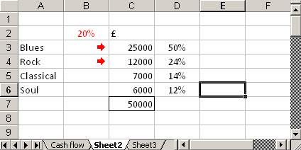
include an additional column designed just to contain a highlight 'pointer' to
cells that we wish to emphasise.
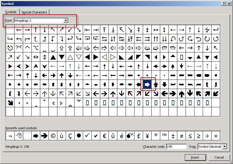
Prior to Excel 2007 you could achieve this by filling your highlight column with the highlight symbol you wish to use. This may involve the use of Insert, Symbol or, prior to Excel XP, copy and paste from Word. You may also need to change the font of the relevant cells to display the symbol correctly.
Now, rather strangely, we change
the colour of the font used in the cells to white to make all the symbols
disappear again.
Next we highlight
the cells containing the invisible symbols and use conditional formatting to
change the font colour to red when our condition for emphasis is met:
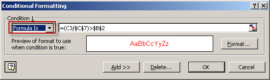
We have used the
'Formula is' type of condition and set the formula to calculate the 'current'
cell as a percentage of the total and compare this with a threshold value held
in B2. Note that the current cell uses relative references so it will adjust for
each of the rows we apply it to.
Excel
2007 only
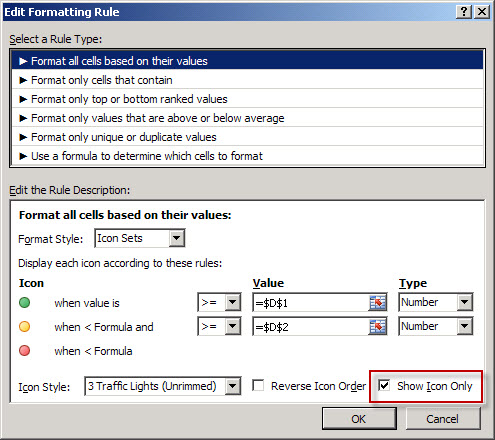
There is an
alternative method in Excel 2007. Here, we enter a formula that calculates our
percentage in the highlight column – D in this case. We then select those
cells and apply a conditional format based on the Format Style 'Icon Sets'. Here
we have used a 3 Traffic Lights approach and based the condition on the values
in cells D1 and D2:
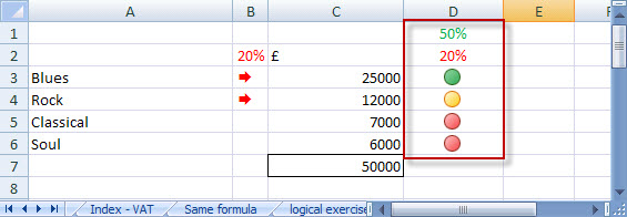
The result is as
shown here:
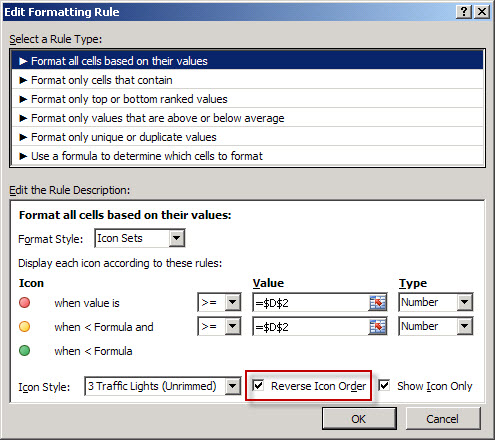
If we needed to match the Excel 2003 approach more closely, We could Reverse the Icon Order in the rule and make the top, red icon apply just to our 20% value - for reasons that will shortly become clear, we don't need to worry about the other two elements of our rule:
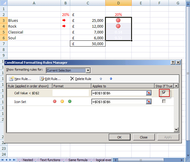
We now set up another rule applied to the same cells. This rule just checks for values below our D2 value and sets the Format to white text on a white background in order to hide the cell values:
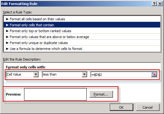
The final step is to ensure that this new rule 'catches' all values below our trigger value, before the traffic light rule allocates different coloured icons to them. We do this by turning on the 'Stop If True' option:
Design by Reading Room Ltd 1998