Search other Office resources (AccountingWeb, Beancounters Guide, IT Counts):

Excel - Convert your overdraft to cash-in-hand

Introduction

This arose from a query at one of our lectures. The task is to link to a set of accounting trial balance data, and automatically convert some account codes to other accounts depending on the value. So, for example, our bank account is '771' when it's a debit balance, but we want it to be '871' when it goes into credit. Firstly, it probably be much easier to do this in a database rather than in Excel, then link Excel to the result, but we'll assume we haven't got a database or that we just want the intellectual challenge of doing it in Excel! Secondly, I'm haunted by the thought that there's a ridiculously simple way of doing this that I haven't thought of...

Approach

The approach we've taken is as follows. We want to make the conversion operation totally automatic, so we don't want the user to have to enter any formulae at all. The data is going to be brought in via a 'Get External Data' link and for the purposes of this article we are just using a very simple text-based CSV (comma separated values) file:

Code,Value
100,-80
200,150
771,-100
872,60

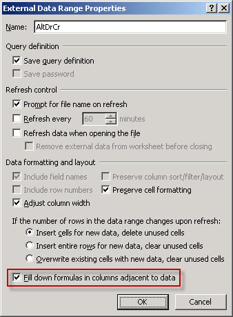
We will link to this file so that we can refresh the data range to bring in new or changed information. We are going to include a column immediately to the right of our linked data that will calculate the correct code to use. In order to ensure that the contents of this column are automatically extended to include any new codes in our source data file, we will turn on the 'Fill down formulas in columns adjacent to data' option in the External Data Range Properties dialog:

The next stage is to create a small table listing the 'changing' codes. This has two columns, the left-hand column lists the debit version of the code and the right-hand column the credit version. It is assumed that the same code will not be entered in both columns!

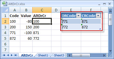
In Excel 2003 this will be set up as a 'List' and in 2007 as a table. This will make it easier to add further Dr/Cr pairings without the need to adjust any formulae. (For more details on how lists and tables work see: http://www.tkb.co.uk/excellist.htm). To make our formula easier to understand, we've given our table the name 'DrCr'. We've placed it immediately next to our data just for demonstration purposes, it would probably be better off on a different sheet.

The formula

Finally, we need to create the formula that will swap the codes as required. This needs to cope with three possibilities:

• Normal code, not included in the Debit/Credit table

• Debit code that needs to be changed to the credit equivalent when value is negative

• Credit code that needs to be changed to the debit equivalent when value is positive

We will use a combination of logical and lookup functions to achieve this. As well as calling the whole table DrCr, we've allocated the range name 'Dr' to the values in the DRCode column and 'Cr' to those in the CRCode column.

First we need to know whether the code is in either column of the table. This is done by using the COUNTIF() function to count the number of occurrences of the code in the whole table:

COUNTIF(DrCr,A2)

This will become the statement in our main IF() function. If the COUNTIF() function returns zero, we know that there is not match in our DrCr table and we can just use the original code.

Assuming there is a match, we need to find whether it's in the DRCode or the CRCode column. First we check the DRCode column. If there is no match the MATCH() function will return N/A so we trap this with the use of the ISNA() function and do nothing. If there is a match, match tells us where it is and we use this information to create an INDEX() function that brings in the corresponding code from the CRCode column,  if the value is negative (B2<0) or sticks with the original code if it is positive (A2):

IF(ISNA(MATCH(A2,Dr,0)),,IF(B2<0,INDEX(DrCr,MATCH(A2,Dr,0),2),A2))

Based on our assumption that the same code shouldn't be in both columns, we then just add the third possibility which is the opposite of our debit test using the concatenation operator '&'

& IF(ISNA(MATCH(A2,Cr,0)),,IF(B2>0,INDEX(DrCr,MATCH(A2,Cr,0),1),A2))

Sticking this all together we get:

=IF(COUNTIF(DrCr,A2)=0,A2,IF(ISNA(MATCH(A2,Dr,0)),,IF(B2<0,INDEX(DrCr,MATCH(A2,Dr,0),2),A2))
&IF(ISNA(MATCH(A2,Cr,0)),,IF(B2>0,INDEX(DrCr,MATCH(A2,Cr,0),1),A2)))

Result

We'll now add a line to our DrCr table, and because it's a table our formula ranges should automatically extend to include the new line. We'll also add a row to our source data:

Code,Value
100,-80
200,150
771,-100
872,60
773,-500

and then refresh our external data range:

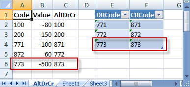
The 'fill down formulas...' option has caused our formula to be copied down to the new row 6 and we can see that the formula has correctly included the row added to our DrCr table.